Rocket Lab

The purpose of this lab was to measure the height of a rocket by using Newton's Second Law. The lab was started by first answering questions that would help us understand what we were about to do. We drew two system schemas, one at rest and one at the moment the rocket leaves the ground. As the fuel of the rocket burned, we knew that the force of thrust has to be greater than the force of gravity, so it can be accelerating up, and since our rocket was not a particle, it would have to deal with air resistance. Since air resistance is not constant, it would increase as the velocity increased. At the point where the rocket runs out of gas, the rocket will still be moving up, but slowing down and reaching it's maximum height.

The second part of the lab was to figure out what specific information and measurements were needed after we had gotten the data of the thrust force of the rocket. The most obvious of the measurements that were needed were the mass, cross sectional area of the rocket, and the force of thrust. From there we came up with equations that would start with the times and thrust that would lead to finding the maximum height of the rocket. The first equation we needed to start off the kinematics was the acceleration that we found by using newton's second law:

a = (Fthrust-Fg-Drag)/m

With the acceleration found, we can find the velocity by using:

V = v +a*delta(t)

With velocity found, we can find the force of drag by using:

D = rhoAv2

And finally, the distance traveled by the rocket could be found by using the position kinematic equation:

R = r + v*delta(t) + .5a*delta(t)

With all the specific information, information, and equations were found, we were able to put it into an excel spreadsheet and had it do all the work for us:

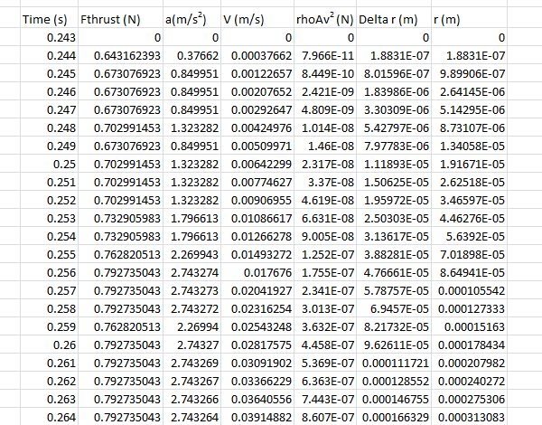
The top excel shows the start time of when the thrust force of the rocket was greater than the force of gravity. Since the change of time was .001 seconds, the change from one cell to the next was not much of a difference. The maximum height of the rocket was found by finding the time where the rocket came to a stop. The time being the average of two: 7.575 s. It's maximum height was also taken by finding the average of two numbers: 147.26 m.

This lab put into effect Newton's second law in that the net force is the sum of all forces action on the object thus the acceleration vector points in the same direction as the force vector. This lab had minimal sources errors in that most measurements were given. The only source of error would be that the equations used to lead up to finding the maximum height were not entirely correct. Another source of error could be that the logger pro failed to accurately record the data of the force of thrust. But since the maximum height was the same as the one the instructor had, errors were minimal. Another great lab would be to use different type of engines, or different sized rockets.

Working with Spreadsheets Lab

The purpose of this lab was to become familiar with electronic spreadsheets by using them in some simple applications by the use of a computer with Excel software.

We were given the values of A =5, B =3, and C = π/3. We placed the values on the left side of the

spreadsheet and labeled them with amplitude, frequency, and phase as an explanation for the meaning of 

each constant. We also made a column for "x" and "f(x)" with "x" being in increments of 0.1 radians and

"f(x)" being this formula:

f(x) = A sin(Bx + C)

With those given values, increments, and formula, we were able to come up with Table #1, and also one that

shows exactly how we applied the formula to the software using the different columns and rows:

Once we were sure all the data was input correctly, we copied and pasted the data onto the Graphical analysis software. A graph of the data appeared and was labeled with correct vertical and horizontal axes. We then directed the computer to find a function that best fits the data which was the same that was used to find "f(x)." The graph was in the form of sin(x):

The values that were given by the computer by using the function that best matched the data, gave the same exact numbers that were used in the spreadsheet to find what "f(x) was equal to. A was equal to 5, B was equal to 3, and C was equal to π/3. The graph had the same amplitude, frequency and phase.

After that first spreadsheet was completed, we repeated the process for a spreadsheet that calculates the position

of a freely falling particle as a function of time. The constants that were included were acceleration of gravity,

the initial velocity, initial position, and the time increment. G = 9.8 m/s^2, v0 =50 m/s, x0 = 1000 m, and Δt = 0.2s. We put our constants on the left side and had two columns of "x" and "f(x)" where we used the quadratic formula:

f(x) = A + Bx + Cx^2

and found how much the particle had fallen for every 0.2 s:

A data table for Data Table #2 was also made that shows how the columns and rows were used for the software to make the calculations for us:

After the data was checked, and was accurate to the constants we were given for the calculations, we copied and pasted column "x" and "f(x)" onto the Graphical Analysis software and labeled the horizontal x-axis and vertical y-axis. The software gave us the shape of a concave up parabola that started from 1000 m, traveled up about 63 m, and them came falling down with an acceleration of 9.8 m/s^2 to 0 m. We then had the computer find a function that best fit the curve which came out the be the quadratic formula that was also used to calculate the data:

The values that the computer gave us for A, B, and C were the same that we had been given from the beginning. The particle had been thrown with an initial velocity of 50 m/s at 1000 m high with a constant acceleration of 9.8 m/s^2. The data that was calculated in the spreadsheet was the same as the data that the Graphical Analysis calculated.

The lab demonstrated how data can be more precisely gathered by the use of software that accurately does calculations. It taught how to input data into Excel, and giving it functions that will use the data you input to solve for whatever is being sought. The lab didn't bring up many sources of error since the software in the computer held the task of doing the calculations. The only error that could have happened could be a slightly small human error in that input of data could have been written wrong or not paired up correctly into the functions. A further thing that the lab could teach is finding derivatives of functions that would help find out how the position vs. time, velocity vs. time, or acceleration vs. time graph would look.

Acceleration of Gravity Lab

The purpose of this lab was to determine the acceleration of gravity for a free falling object, and to become literate with the equipment that was use to collect the data. We were shown how to set up the equipment, and how to accurately throw the object so the sound waves given off by the motion detector capture the motion of object as it is thrown up and falls back down.

We first set up the software and opened up the program that would be recording the motion of the ball. We were to throw the ball above the motion detector and let it fall back down on to the motion detector. We practiced for a couple tries and then started recording our trials until we had a position vs. time graph and a velocity vs. time graph that had the least amount of error which was these:

The velocity vs. time graph gave us a parabola because as the ball moved away from the motion detector, it was increasing till it came to a stop which would be the maximum of the parabola, and then the ball started to fall back down towards the motion detector which would mean it was decreasing. We were able to find the values of a, b, and c by using the quadratic formula:

x=At^2+Bt=C

The quadratic formula gave us the value of A(4.94) which we multiplied by 2 to give us our measured acceleration of gravity that came out to 9.88m/s^2. We then calculated the percent error by using this equation:

Percent Error= (measured-actual/actual)*100

The percent error that the formula was .816%, so our calculation wasn't that much off.

For the velocity vs. time graph we found the values of m and b using a linear fit to find the slope that would give us our measured acceleration of gravity which was 10.2m/s^2. We used the same function as the other graph to find the percent error which was 4.082%. The velocity versus time graph was also not far from being the actual accepted value of 9.8m/s^2 for the acceleration of gravity.

Vector Lab

               Figure 1: The sum of Vector 1 and Vector 2 equal Vector 3.